
What is the purpose of a Marine Protected Area?
Marine Protected Areas (or MPAs) endeavor to protect marine life and crucial marine habitats for both their intrinsic and cultural values. While MPAs are discrete geographic regions characterized by regulations limiting or entirely preventing human interaction, they support a wide array of organisms that may be transient between multiple areas (protected or non).
Desires to protect or preserve local fisheries often play a major role in motivating MPA development. As a result, fishery species biomass is of special interest to policy makers, who allocate funds and advise the management of these areas.
As of 2025, MPA networks are utilized worldwide, but there is no unified methodology for determining how MPAs affect key species biomass. This is due in part to the difficulty in establishing a counterfactual that MPA sites can be compared to, in order to ascertain the trajectory of key species biomass in the absence of MPA establishment in these areas.
MPA boundaries are often selected to encompass specific biota and biodiversity, and thus are not randomly selected. Since marine monitoring and research is time consuming and costly, it is highly unlikley that there will be legacy monitoring of a region before it becomes an MPA.
However, there have been some promising frameworks proposed that utilized sites with legacy monitoring to test the validity of their proposed designs.
How can we measure their effectiveness?
In the paper “Integrating impact evaluation in the design and implementation of monitoring marine protected areas” by Ahmadiyya et al. 2015 1, the researchers suggested that proposed sites should be randomly selected and monitored before the time of MPA establishment, to act as counterfactuals for future analysis of MPA effectiveness. If this were not possible with time constraints, then control sites should be randomly selected and paired to MPA sites before establishment and continually be monitored. They stated that a wide array of environmental and anthropogenic factors should be monitored in both the control and MPA sites to better evaluate each system, their sentiments best stated in the quote:
“To inform decisions about MPA placement, design and implementation, we need to expand our understanding of conditions under which MPAs are likely to lead to positive outcomes by embracing advances in impact evaluation methodologies” (Ahmadiyya et al. 2015)
They then proposed using a coarse and statistical matching with a Difference-in-Difference (DiD) method for analyzing key fisheries species biomass, as well as functional species biomass (herbivorous fish that maintain the reef) between sites. After this, their main objective was to utilize a hierarchical mixed effects model would be used to determine how each variable contributes to key species biomass, and how they interact with one another.
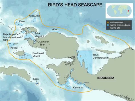
To demonstrate the application of this framework, they decided to select a pre-existing MPA site with a plethora of monitoring data, Bird’s Head Seascape in Indonesia, and “reverse engineer” counterfactual sites in order to run DiD and hierarchical mixed effects models.
This was accomplished via the selection of 10 primary covariates, selected by local researchers and reef specialists, comprehensive literature reviews, and determining what aligned with available data. The researchers affirmed that their covariates ” The final covariates were determined to encompass “structural, biophysical, and social features of coral-reef sites that influence ecosystem structure”.
Due to limitations in the sampling, with only one year of pre-MPA establishment data to utilize for the DiD analysis, the researchers decided to do a “post-hoc regression adjustment” that will use more data and decrease unobserved bias in the coming years.
Difference-in-Difference (DiD)
A type of “Before-After Control-Impact” (BACI) analysis with an ecological focus, a Difference-in-Difference study leverages time trends when random assignment is not possible. Essentially, you can compare the same site before and after the implementation of the treatment to determine if it had any effect. DiD studies often use a linear regression to accomplish this.
A couple of the key assumptions made in using this model are :
The baseline outcome would have persisted unchanged over time
Parallel trends exist pre-treatment
This process involves both coarse and statistical matching. Coarse matching involves grouping the sites by common physical, chemical, and ecological attributes by researchers, informed by experts in coral reef ecology (reefs with similar coral diversity, similar wave action, reef type, etc.).
Hierarchical Mixed Effect Model
Statistical matching involved utilizing a hierarchical mixed effects model to cluster control sites and MPA sites. The researchers used nearest-neighbor covariate matching to create grouped sites with similar traits.
The Mahalanobis distance metric was used to find the smallest mean differences between distributions of covariates across treated and control sites. All 10 covariates were weighted equally, and had calipers applied to them to ensure sites were grouped by similar traits (slope reefs only grouped with slope reefs, high risk only grouped with high rick, etc.).
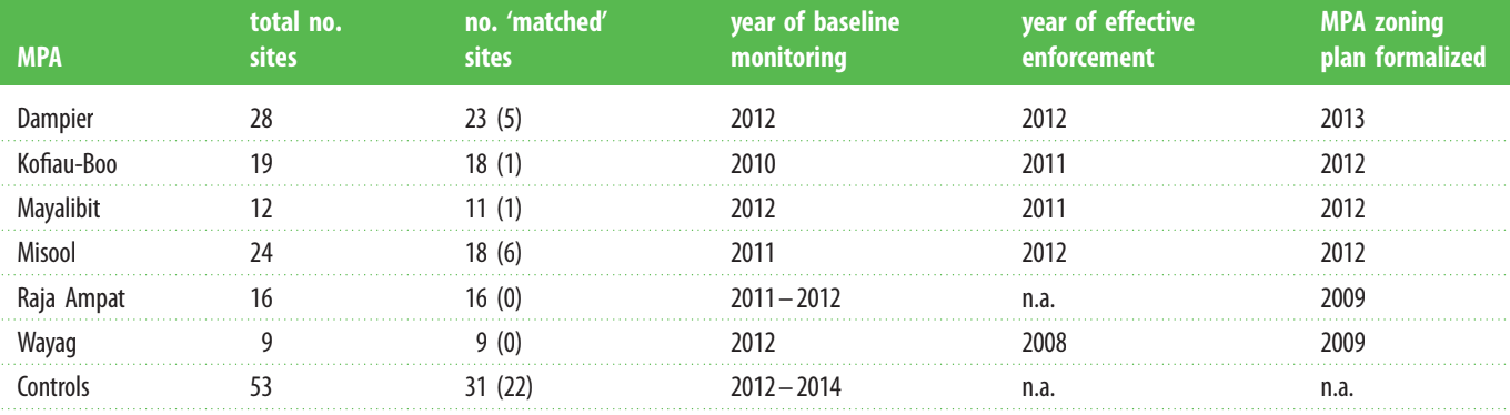
After multiple iterations considering the trade-offs between dropped MPA sites and achieving covariate balance, the optimal matching model dropped 13 of the 108 MPA sites and 22 of the 53 control sites.

Primary Covariates
The 10 primary covariates for this study were:
Reef Type (‘patch’, ‘fringe’, ‘barrier’, ‘atoll’)
Reef Slope (site identified as ‘flat’, ‘slope’, or ‘wall’)
Reef Exposure (exposed to air & increased wave energy: identified as ‘exposed’, ‘semi-exposed’,‘sheltered’)
Pollution risk (Erosion rates, sediment delivery, sediment trapping, and sediment dispersal modeled and rated as ‘low’, ‘medium’, or ‘high’ threat level.)
Monsoon direction (Reefs faced north or westerly exposed to northwest monsoon winds, while reefs facing south and easterly are exposed to southeast monsoon winds. Exposure to currents, wind, and precipitation is assumed to be similar in each group.
Sea-surface temperature anomalies (SSTA: “Number of times over the previous 52 weeks that SST was greater than or equal to 1 degree Celsius above that week’s long term average value”)
Distance to market
Distance to fishing settlement
Distance to deep water
Distance to mangrove habitat
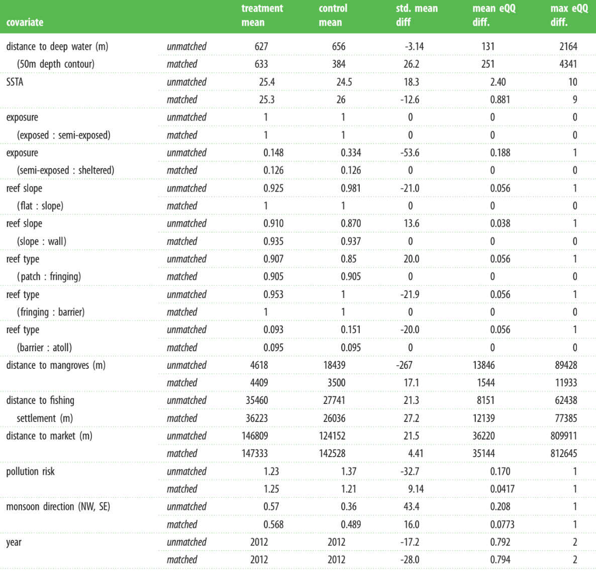
Standardized mean differences of less than 5% for a covariate are typically necessary for robust causal inference. While 6 of these covariates met the threshold, the last 4 did not. This suggests that, on average, MPA sites are further from markets, fishing settlements, mangroves, and deep water as compared to control sites, indicating that MPA sites are more “cherry-picked” than the controls.
In order to address this, these 4 covariates need to be accounted for in the post-hoc analysis to avoid omitted variable bias.

Findings
Using only their initial DiD results (post-hoc regression adjustment has not occurred yet), their main findings showed that in the pooled data for all MPAs we see an increase in specifically fisheries biomass, while functional group (smaller herbivorous fish) biomass remains unchanged from predicted baseline.
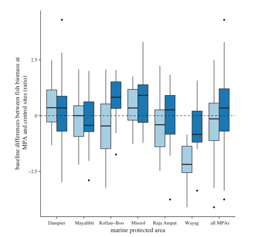
While there is not much to extrapolate from this analysis, we believe that the authors summed it up rather well when they said “We anticipate that the value of this baseline data, now combined with control site data, will only increase with time. And as more geographies use comparable monitoring methods and well-designed sampling”
Robustness & Application
For their robustness check, the authors specifically wanted to analyze unobserved biases in the model via sensitivity analysis. They referenced an analysis format which uses M-estimators (such as least-squares, maximum likelihood estimation, and confidence intervals) to reduce omitted variable bias.
However, it should be noted that this analysis has not been performed yet, as they are still waiting to complete further post-hoc analysis once they have more data.
The researchers stated that, in reference to “observable biases that cannot be adequately controlled by our statistical matching model” (e.g. distance to fishing settlement, mangrove habitat and deep water, and year which did not have a standard difference of less than 5%), “we account for the magnitude and direction of this bias in our mixed model, in a procedure known as post-hoc regression adjustment”.
Overall, due to the in depth selection and comparison of covariates to reduce observed bias, and the researchers not overextending the applicability of their data by sticking to a nearest-neighbor matching and Difference-in-Difference model, means their findings are robust, and present a convincing argument for the application of their MPA monitoring framework.
I personally look forward to further publications from these authors, to see how well this framework holds up in the future with increased sampling of MPAs and control sites.
Footnotes
Ahmadia, G. N., Glew, L., Provost, M., Gill, D., Hidayat, N. I., Mangubhai, S., Purwanto, & Fox, H. E. (2015). Integrating impact evaluation in the design and implementation of monitoring marine protected areas. Philosophical transactions of the Royal Society of London. Series B, Biological sciences, 370(1681), 20140275. https://doi.org/10.1098/rstb.2014.0275. Link to article↩︎